DynamoDB is a truly unique and powerful database. It provides a predictable low latency, a vast array of features, tight integration with other AWS services and almost no operational load.

The only problem is that its data model can seem bizarre. The moment you start learning about it you will stumble upon partition keys, global secondary indexes, and other unusual concepts. Where would you even begin?

In this article, I will explain how to use core DynamoDB features to and how to fit your data into it. To be more practical I will show how to create a simple database that stores information about videos on a video sharing website.

Data in DynamoDB

Before we start designing data store for our application, let’s talk about how data is organized in DynamoDB. The most high-level element in DynamoDB is a table. When you work with data in DynamoDB, you work with a single table, and there are no operations that span multiple tables. In this article, I will call a logical group of tables a database, but there is no special support for this in DynamoDB.

 

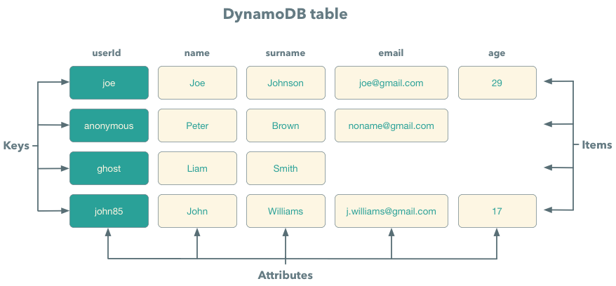
Every table is a collection of items, and every item is a collection key/value pairs called attributes. In contrast to relational databases, DynamoDB does not enforce a strict schema. It means that different items can have different numbers of attributes and attributes with the same name can have different types. Every item should have a total size less than 400KB.

The only exception to this rule is a key attribute. Every item in a database should have a key DynamoDB enforces a type of key attributes.

DynamoDB supports several data types that can be divided into scalar types, set types, and document types. Scalar types include:

• String – a UTF-8 string, and is only limited by the maximum size of an item
• Number – a float point number that can have up to 38 digits precision
• Binary – an array of unsigned bytes that is limited by the maximum size of an item
• Boolean – true or false values
• Null – for unknown or undefined state

// Scalar types item
{
    "videoId": "rk67v9",
    "name": "How to make pancakes",
    // Binary image represented as Base64
    "featuredImage": "ab4f...86ty", 
    "videoFile": ,
    "length": 3786,
    "published": true,
    "rating": null
}

Set types, just as the name suggest, are special types for sets. DynamoDB supports sets of Strings, Numbers and Binary values. These sets do not store duplicate values and do not preserve order. Surprisingly, DynamoDB does not support an empty set.

Lastly, there are only two document types in DynamoDB:

• Map – a nested data structure similar to a JSON object
• List – an ordered sequence of elements on any types

// Document types
{
    "movieId": "123",
    "name": "Star Wars: The Force Awakens",
    "actors": [
        "Daisy Ridley",
        "John Boyega",
        ...
    ],
    "boxOffice": {
        "budget": 245000000,
        "gross": 936000000
    }
}

Mind the price

When you create a table, you need to specify how many requests a table should be able to process per second. The more requests you need to process the more you will have to pay. Hence it pays to understand how we can use as little provisioned throughput as possible.

A table throughput is defined by two values:

• Number of read capacity units (RCUs) – how many read requests can you send per second.
• Number of write capacity units (WCUs) – how many write requests can you send per second.

Not all requests are equal though. The more data you read or write in a single request, the more read and write capacity will be consumed. The calculation looks like this:

RCU_consumed = ceil(size_read / 4KB)
WCU_consumed = ceil(size_written / 1KB)

You can change the provisioned throughput at any time by performing the UpdateTable API call. If you send more requests to the table than it can handle DynamoDB will return the ProvisionedThroughputExceededException exception, and you need either to retry or provision more capacity.

Another thing to keep in mind is that you can use two types of read operations: eventual.y consistent and strongly consistent. With strongly consistent read you are guaranteed to get the latest written result. With eventual consistency, you can get stale data, but it will consume twice less capacity units than a strongly consistent read.

Table keys and how to select them

Simple key

Now, let’s go back to our videos database. Let’s design a first table that will store information about video authors such as user id, name, country, and most importantly: a favourite beverage. But before we can store out first item DynamoDB forces to make an important choice: we need to select what field(s) will form a key in our table. This choice is important for two reasons: first of all this defines what queries we can perform efficiently and second you can’t change it after the table is created.

For the video authors table, we will use a so-called simple key. With the simple key a single attribute is defined as a key in the table:

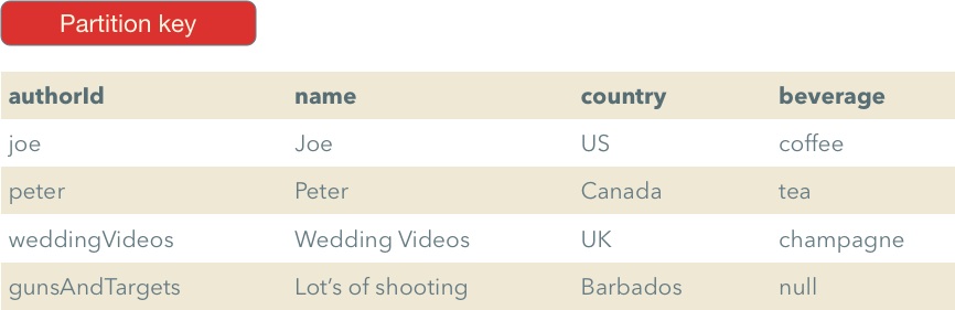
With this key type we can perform only one query efficiently: get an item by id. To do this, we need to use the GetItem action.

In addition to that, you can use an operation called Scan to fetch your data. Scan allows to provide an arbitrary filtering expression which allows great flexibility, and this can make you wonder why do we need to care about key types in the first place. The problem is that when you use Scan DynamoDB consumes capacity for every item DynamoDB evaluates even if it does not return it to you. And since Scan operation does not use any knowledge about the structure of your data using it on a big table can be really expensive.

A simple key is fine for simple cases, but it’s hard to implement something more complicated than this. Say we want to implement a 1:M relationship authors and videos. We could store a list of videos IDs in a list in an author’s item and then fetch every video using the GetItem action but this is not convenient and not cost-efficient.

// Possible solution
{
    "authorId": "unclebob",
    "videos": ["sd82s7", "whd2bs", ..., "ful57s"]
}

If we call GetItem to get a number of items we spend at least one RCU for every call even if a size of an item is less than 4KB. So if we want to fetch ten items 400 bytes each, it will cost us 10 RCUs!

Complex key

There is, however, a better way. DynamoDB has a different key type which is called a composite key. When we create a table with a composite key, we need to define two attributes: a partition key and a sort key. As the name suggests the sort key can be used to sort the output, but it can also do much more.

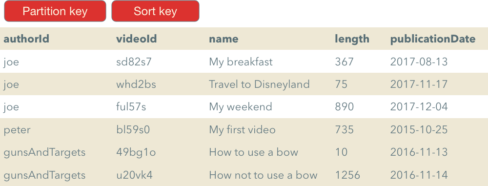
Just as with the simple key you can get an element by id, but in this case you need to provide two values for both simple and sort keys. You can also get all items with the same partition key if use the Query action and only provide the partition key. This is very convenient to implement 1:M relationships.

Optionally with the Query operation, you can provide a key condition expression that allows filtering items in the response. To do this you can use <, >, <=, >=, BETWEEN, and begins_with operators.

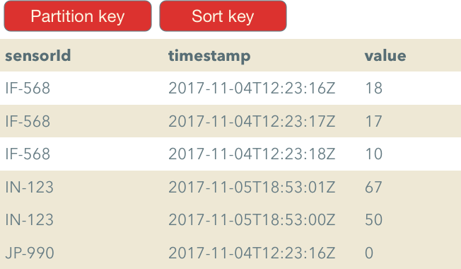
Also, you can specify a sort order based on the sort key value. This does not make much sense with our videos table but it would make more sense in a different case. Say, if we have a table where we store sensor measurements we could make sensor id a partition key and a timestamp of a measurement a sort key. With this, we could sort or filter measurements for a particular sensor by timestamp.

Using a sort key it is also easy to paginate requests. All we need to do is to specify the Limit parameter that limits the number of item DynamoDB should evaluate before returning a reply.

Notice that queries with composite keys only operate with values for a single partition key.

Consumed capacity

Remember the issue with consuming too much read capacity using the GetItem action? This is not the case with the query operation. Now if we want to get ten items 400 bytes each it will only cost us 1 RCU. The reason for this is that when we use queries DynamoDB sums the total size of all returned items and only then divides them by 4KB to calculate the consumed capacity:

consumed_capacity = ceil(sum(item_sizes) / 4KB)

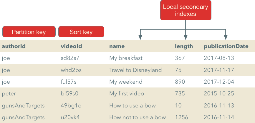
Local secondary index

You can see that the complex key is a very powerful construct, but what if we want to have more than one sort order? What if we want to sort item by a video lengths or by a release date?

For this DynamoDB has another feature called local secondary index. We can use it just like the sort key and can use comparison operators and specify a sort order. For example, if we need to sort videos by video length we can add a local secondary index.

With this approach, we can now sort videos by a particular author by time creation, fetch video created only after some date, filter videos that are longer than some threshold, etc. An important difference compared to the sort key is that a pair of partition key/local secondary index attribute should not be unique.

Notice that when you perform a query, you can use either a sort key or one of the local secondary indexes and not both. Just as with the key type you have to specify local secondary indexes on table creation and can’t change them afterward.

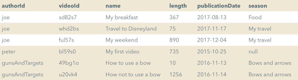
Global secondary index

In previous examples we had tables with a single partition key. This is not very convenient since we can only use the Query operation to fetch items with a selected partition key. What if we want to allow authors to group videos in seasons and want to fetch all videos in a season:

One option would be to maintain a copy of this data in a different table with a different partition key, but the same sort key.

Fortunately, DynamoDB can do this for us. If you create a globally secondary index for a table, you can specify an alternative simple or composite key regardless of what key type you selected for the table. When you write an item into the original item DynamoDB will copy data in the background into the global secondary index table:

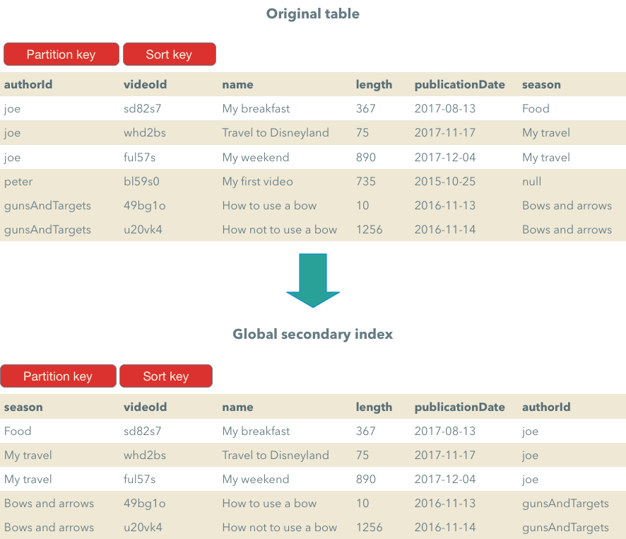
Because data is copied to the index in the background, it only supports eventually consistent read operations. This is because it takes some time for updates to propagate.

In contrast to local secondary indexes, global secondary indexes can be created at any time even after the table was created.

Aggregating data with DynamoDB

But what if we need to group items by some key with DynamoDB? What if we want to count how many videos do we have from each author? Or what if we need to find out how many videos from 5 to 10 minutes long do we have?

With a relational database we could use the GROUP BY operation, but unfortunately, DynamoDB does not support it out of the box. We have three main options of how we can implement it:

• Use Redshift integration – we can copy data from DynamoDB to Redshift that has a full-fledged SQL support and allows to perform analytical queries. The main downside of this approach is that we will have to query stale data.
• Use EMR Hive integration – with this we can either copy DynamoDB data to HDFS or S3 and query data from there or, alternatively, EMR Hive can perform analytical queries on DynamoDB data itself.
• Create aggregated tables with DynamoDB streams – we can create some sort of a materialized view of original data that fits DynamoDB data model. To maintain this materialized view, we read data from DynamoDB streams, and update materialized view in real time.

Conclusions

While the data model of DynamoDB can seem peculiar at first, it is actually pretty straightforward. Once you’ve grasped what table keys are and how to use table indexes, you will be able to efficiently use DynamoDB. The key is to understand its data model and to think how you can fit your data in DynamoDB. Remember. To achieve the stellar performance you need to use queries as much as possible and try to avoid scan operations.

DynamoDB is a complex topic, and I will write more about it, so so stay tuned. In the meantime, you can take a look at my deep dive DynamoDB course. You can watch the preview for the course here.